Uk Elections 2024

Well I did say I’d do another one of these come the next UK election, so here goes. The official data won’t be published until Friday the 12th of July but we can use our creativity to get it before then. Ok, I did so you don’t have to and you can get the results here.

I’d ideally like to make use of parlitools’ west_hex_map, as I did previously, but unfortunately that package is out of date with respect to the electoral areas of the UK. After a bit of searching, I did find a new hex map for this purpose here – thank you Alasdair Rae & co. Alasdair also explains why you might want to use these hex maps instead of a regular geographically-accurate map in this blogpost (equal population areas).

I’ll combine this hex with the election results linked to above through the GSS Code. You can get this data from here.

First, we’ll load the libraries I’m going to use and get the data we need.

library(ggplot2)
library(sf)
library(dplyr)
library(purrr)
library(jsonlite)

results_data <- "https://raw.githubusercontent.com/RobertMyles/blogdata/master/uk_elections_2024.json"
hexes <- st_read("https://automaticknowledge.org/wpc-hex/uk-wpc-hex-constitcode-v5-june-2024.geojson", quiet = TRUE)

The results are in a list, so I will use pluck() from the purrr package to take out the actual results (constit_summary ) and the full party name (sop > parties). I’m going to rename some columns here to make joining easier later on.

parties <- fromJSON(results_data) |> 
  pluck("sop", "parties") |> 
  select(party = name, party_abb = abbreviation)

results <- fromJSON(results_data) %>%
  pluck("constit_summary") |> 
  rename(party_abb = winner_abbreviation) |> 
  left_join(parties) |> 
  mutate(
    party = case_when(
      party_abb == "TUV" ~ "The Unionist Voice",
      party_abb == "Ind" ~ "Independent",
      party_abb == "Speaker" ~ "Speaker",
      TRUE ~ party
    )
  )

hexes <- hexes |> rename(pcon24 = GSScode)

Ok, so now we can have a quick look at the results (Labour smashed the Conservative party, in case you didn’t know).

results |> 
  group_by(party) |> 
  count(sort = TRUE)

# A tibble: 15 × 2
# Groups:   party [15]
   party                                  n
   <chr>                              <int>
 1 Labour                               411
 2 Conservative                         121
 3 Liberal Democrat                      71
 4 Scottish National Party                9
 5 Sinn Fein                              7
 6 Independent                            6
 7 Democratic Unionist Party              5
 8 Green                                  4
 9 Plaid Cymru                            4
10 Reform UK                              4
11 Social Democratic and Labour Party     2
12 Alliance                               1
13 Speaker                                1
14 The Unionist Voice                     1
15 Ulster Unionist Party                  1

So we’ve got a few small parties here, and the Speaker. Let’s group them into an “Other” category.

results <- results |> 
  mutate(
    party = case_when(
      party_abb %in% c("Alliance", "Speaker", "UUP", "SDLP", "TUV") ~ "Other",
      TRUE ~ party
      )
    )

Our election data looks pretty good now so we can join it with the hex map data. There are two constituencies that haven’t declared at the time of writing so we’ll remove those.

map <- hexes |> left_join(results, by = "pcon24")

map <- map |> 
  filter(!is.na(party)) %>%
  st_as_sf()

Let’s plot ’er up! (Colour scheme from here)

ggplot(map) +
  geom_sf(aes(fill = party), size = 0.2) +
  theme_void() +
  guides(fill = guide_legend(title = "Party", position = "left")) +
  scale_fill_manual(values = c(
     "#5691AF", "#975654", "#72A768", "#98B3D1", 
     "#DA5C5B", "#E0AD3B", "#888888", "#9DCB84",
     "#54B3CC", "#F1D848", "#5A9464"
     )
    )

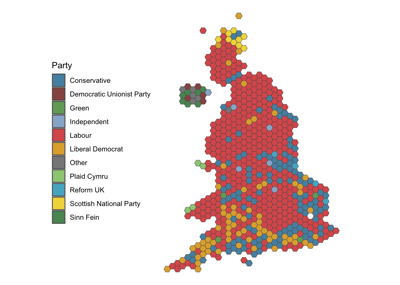
Very different to last time!